🙌 The Hitchhiker’s Guide to Machine Learning in Python

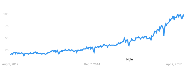
The Trend

Machine learning is undoubtedly on the rise, slowly climbing into ‘buzzword’ territory. This is in large part due to misuse and simple misunderstanding of the topics that come with the term. Take a quick glance at the chart below and you’ll see this illustrated quite clearly thanks to Google Trends’ analysis of interest in the term over the last few years.

The Goal

However, the goal of this article is not to simply reflect on the popularity of machine learning. It is rather to explain and implement relevant machine learning algorithms in a clear and concise way. If I am successful then you will walk away with a little better understanding of the algorithms or at the very least some code to serve as a jumping off point when you go to try them out for yourself.

The Breakdown

I will be covering a total of 8 different machine learning algorithms (with more to come). Feel free to jump around or skip an algorithm if you’ve got it down. Use this guide however your heart desires. So without further adieu, here’s how it’s broken down:

1. Linear Regression
2. Logistic Regression
3. Decision Trees
4. Support Vector Machines
5. K-Nearest Neighbors
6. Random Forests
7. K-Means Clustering
8. Principal Components Analysis

Housekeeping

I’m including this simply because this is one of my pet peeves. Trying to utilize someone else’s code only to find that you need three new packages and the code was run in an older version of your language is incredibly frustrating.

So in the interest of making both of our lives easier, I am using Python 3.5.2and below are the packages I imported prior to these exercises. I also took my sample data from the Diabetes and Iris datasets within the UCI Machine Learning Repository. Lastly, if you want to skip all this and just see all the code, feel free to give it a look on Github.

Linear Regression

Explained

Perhaps the most popular machine learning algorithm out there and definitely the most under appreciated. Many data scientists have a tendency to forget that simpler is almost always preferred over complex when performance is comparable.

Anyways, linear regression is a supervised learning algorithm that predicts an outcome based on continuous features. Linear regression is versatile in the sense that it has the ability to be run on a single variable (simple linear regression) or on many features (multiple linear regression). The way it works is by assigning optimal weights to the variables in order to create a line (ax + b) that will be used to predict output. Check out the video below for a more thorough explanation.

Now that you’ve got a grasp on the concepts behind linear regression, let’s go ahead and implement it in Python.

Getting Started

from sklearn import linear_model
df = pd.read_csv(‘linear_regression_df.csv’)
df.columns = [‘X’, ‘Y’]
df.head()

Visualization

sns.set_context(“notebook”, font_scale=1.1)
sns.set_style(“ticks”)
sns.lmplot(‘X’,’Y’, data=df)

Implementation

linear = linear_model.LinearRegression()
trainX = np.asarray(df.X[20:len(df.X)]).reshape(-1, 1)
trainY = np.asarray(df.Y[20:len(df.Y)]).reshape(-1, 1)
testX = np.asarray(df.X[:20]).reshape(-1, 1)
testY = np.asarray(df.Y[:20]).reshape(-1, 1)
linear.fit(trainX, trainY)
linear.score(trainX, trainY)
print(‘Coefficient: \n’, linear.coef_)
print(‘Intercept: \n’, linear.intercept_)
print(‘R² Value: \n’, linear.score(trainX, trainY))
predicted = linear.predict(testX)

Logistic Regression

Explained

Logistic regression is a supervised classification algorithm and therefore is useful for estimating discrete values. It is typically used for predicting the probability of an event using the logistic function in order to get an output between 0 and 1.

When first learning this logistic regression, I was under the impression that it was a sort of a niche thing and therefore I didn’t give it my full attention. In hindsight, I couldn’t have been more wrong. Some of the underlying aspects of logistic regression come up in many other important machine learning algorithms like neural networks. With this in mind, go ahead and check out the video below for more.

Now that you’ve got a grasp on the concepts behind logistic regression, let’s implement it in Python.

Getting Started

from sklearn.linear_model
import LogisticRegression
df = pd.read_csv(‘logistic_regression_df.csv’)
df.columns = [‘X’, ‘Y’]
df.head()

Visualization

sns.set_context(“notebook”, font_scale=1.1
sns.set_style(“ticks”)
sns.regplot(‘X’,’Y’, data=df, logistic=True)
plt.ylabel(‘Probability’)
plt.xlabel(‘Explanatory’)

Implementation

logistic = LogisticRegression()
X = (np.asarray(df.X)).reshape(-1, 1)
Y = (np.asarray(df.Y)).ravel()
logistic.fit(X, Y)logistic.score(X, Y)
print(‘Coefficient: \n’, logistic.coef_)
print(‘Intercept: \n’, logistic.intercept_)
print(‘R² Value: \n’, logistic.score(X, Y))

Decision Trees

Explained

Decision trees are a form of supervised learning that can be used for both classification and regression purposes. In my experience, they are typically utilized for classification purposes. The model takes in an instance and then goes down the tree, testing significant features against a determined conditional statement. Depending on the result, it will go down to the left or right child branch and onward after that. Typically the most significant features in the process will fall closer to the root of the tree.

Decision trees are becoming increasingly popular and can serve as a strong learning algorithm for any data scientist to have in their repertoire, especially when coupled with techniques like random forests, boosting, and bagging. Once again, use the video below for a more in-depth look into the underlying functionality of decision trees.

Now that you know a little more about decision trees and how they work, let’s go ahead and implement one in Python.

Getting Started

from sklearn import tree
df = pd.read_csv(‘iris_df.csv’)
df.columns = [‘X1’, ‘X2’, ‘X3’, ‘X4’, ‘Y’]
df.head()

Implementation

from sklearn.cross_validation
import train_test_split
decision = tree.DecisionTreeClassifier(criterion=’gini’)
Y = df.values[:, 4]
trainX, testX, trainY, testY = train_test_split( X, Y, test_size = 0.3)
decision.fit(trainX, trainY
print(‘Accuracy: \n’, decision.score(testX, testY))

Visualization

from sklearn.externals.six import StringIO
from IPython.display import Image
from IPython.display import Image
import pydotplus as pydotdot
data = StringIO()
tree.export_graphviz(decision, out_file=dot_data)
graph = pydot.graph_from_dot_data(dot_data.getvalue())
Image(graph.create_png())

Support Vector Machines

Explained

Support vector machines, also known as SVM, are a well-known supervised classification algorithm that create a dividing line between the your differing categories of data. The way this vector is calculated, in simple terms, is by optimizing the line so that the closest point in each of the groups will be farthest away from each other.

This vector is by default and often visualized as being linear, however this doesn’t have to always be the case. The vector can take a nonlinear form as well if the kernel type is changed from the default type of ‘gaussian’ or linear. There’s much more to be said about SVM, so be sure to look into the instructional video below.

Now that you know all about support vector machines, let’s go ahead and implement them in Python.

Getting Started

from sklearn import svm
df = pd.read_csv(‘iris_df.csv’)
df.columns = [‘X4’, ‘X3’, ‘X1’, ‘X2’, ‘Y’]
df = df.drop([‘X4’, ‘X3’], 1)
df.head()

Implementation

from sklearn.cross_validation import train_test_split
df.head()
support = svm.SVC()
X = df.values[:, 0:2]
Y = df.values[:, 2]
trainX, testX, trainY, testY = train_test_split( X, Y, test_size = 0.3)
support.fit(trainX, trainY)
print(‘Accuracy: \n’, support.score(testX, testY))
pred = support.predict(testX)

Visualization

sns.set_context(“notebook”, font_scale=1.1)
sns.set_style(“ticks”)
sns.lmplot(‘X1’,’X2', scatter=True, fit_reg=False, data=df, hue=’Y’)
plt.ylabel(‘X2’)
plt.xlabel(‘X1’)

K-Nearest Neighbors

Explained

K-Nearest Neighbors, KNN for short, is a supervised learning algorithm specializing in classification. The algorithm looks at different centroids and compares distance using some sort of function (usually Euclidean), then analyzes those results and assigns each point to the group so that it is optimized to be placed with all the closest points to it. Check out the video below for much deeper dive into what’s really going on behind the scenes with K-Nearest Neighbors.

Now that you’ve got a grasp on the concepts behind the K-Nearest Neighbors algorithm, let’s implement it in Python.

Getting Started

from sklearn.neighbors import KNeighborsClassifier
df = pd.read_csv(‘iris_df.csv’)
df.columns = [‘X1’, ‘X2’, ‘X3’, ‘X4’, ‘Y’]
df = df.drop([‘X4’, ‘X3’], 1)
df.head()

Visualization

sns.set_context(“notebook”, font_scale=1.1)
sns.set_style(“ticks”)
sns.lmplot(‘X1’,’X2', scatter=True, fit_reg=False, data=df, hue=’Y’)
plt.ylabel(‘X2’)
plt.xlabel(‘X1’)

Implementation

from sklearn.cross_validation import train_test_split
neighbors = KNeighborsClassifier(n_neighbors=5)
X = df.values[:, 0:2]
Y = df.values[:, 2]
trainX, testX, trainY, testY = train_test_split( X, Y, test_size = 0.3)
neighbors.fit(trainX, trainY)
print(‘Accuracy: \n’, neighbors.score(testX, testY))
pred = neighbors.predict(testX)

Random Forests

Explained

Random forests are a popular supervised ensemble learning algorithm. ‘Ensemble’ means that it takes a bunch of ‘weak learners’ and has them work together to form one strong predictor. In this case, the weak learners are all randomly implemented decision trees that are brought together to form the strong predictor — a random forest. Check out the video below for much more behind the scenes stuff regarding random forests.

Now that know all about what’s going on with random forests, time to implement one in Python.

Getting Started

from sklearn.ensemble import RandomForestClassifier
df = pd.read_csv(‘iris_df.csv’)
df.columns = [‘X1’, ‘X2’, ‘X3’, ‘X4’, ‘Y’]
df.head()

Implementation

from sklearn.cross_validation import train_test_split
forest = RandomForestClassifier()
X = df.values[:, 0:4]
Y = df.values[:, 4]
trainX, testX, trainY, testY = train_test_split( X, Y, test_size = 0.3)
forest.fit(trainX, trainY)
print(‘Accuracy: \n’, forest.score(testX, testY))
pred = forest.predict(testX)

K-Means Clustering

Explained

K-Means is a popular unsupervised learning classification algorithm typically used to address the clustering problem. The ‘K’ refers to the user inputted number of clusters. The algorithm begins with randomly selected points and then optimizes the clusters using a distance formula to find the best grouping of data points. It is ultimately up to the data scientist to select the correct ‘K’ value. You know the drill, check out the video for more.

Now that know more about K-Means clustering and how it works, let’s implement the algorithm in Python.

Getting Started

from sklearn.cluster import KMeans
df = pd.read_csv(‘iris_df.csv’)
df.columns = [‘X1’, ‘X2’, ‘X3’, ‘X4’, ‘Y’]
df = df.drop([‘X4’, ‘X3’], 1)
df.head()

Implementation

from sklearn.cross_validation import train_test_split
kmeans = KMeans(n_clusters=3)
X = df.values[:, 0:2]
kmeans.fit(X)
df[‘Pred’] = kmeans.predict(X)
df.head()

Visualization

sns.set_context(“notebook”, font_scale=1.1)
sns.set_style(“ticks”)
sns.lmplot(‘X1’,’X2', scatter=True, fit_reg=False, data=df, hue = ‘Pred’)

Principal Components Analysis

Explained

PCA is a dimensionality reduction algorithm that can do a couple of things for data scientists. Most importantly, it can dramatically reduce the computational footprint of a model when dealing with hundreds or thousands of different features. It is unsupervised, however the user should still analyze the results and make sure they are keeping 95% or so of the original dataset’s behavior. There’s a lot more to address with PCA so be sure to check out the video for more.

Now that know more about PCA and how it works, let’s implement the algorithm in Python.

Getting Started

from sklearn import decomposition
df = pd.read_csv(‘iris_df.csv’)
df.columns = [‘X1’, ‘X2’, ‘X3’, ‘X4’, ‘Y’]
df.head()

Implementation

from sklearn import decomposition
pca = decomposition.PCA()
fa = decomposition.FactorAnalysis()
X = df.values[:, 0:4]
Y = df.values[:, 4]
train, test = train_test_split(X,test_size = 0.3)
train_reduced = pca.fit_transform(train)
test_reduced = pca.transform(test)
pca.n_components_

Wrapping Up

This tutorial simply scrapes the surface of all the machine learning algorithms being used out there today. With this being said, I hope some of you will find it helpful on your journey to machine learning mastery. To check out the full Jupyter notebook, see my Github

Thanks for reading! If you enjoyed this post and you’re feeling generous, perhaps follow me on Twitter. You can also subscribe in the form below to get future posts like this one straight to your inbox. 🔥